- About MAA
- Membership
- MAA Publications
- Periodicals
- Blogs
- MAA Book Series
- MAA Press (an imprint of the AMS)
- MAA Notes
- MAA Reviews
- Mathematical Communication
- Information for Libraries
- Author Resources
- Advertise with MAA
- Meetings
- Competitions
- Programs
- Communities
- MAA Sections
- SIGMAA
- MAA Connect
- Students
- MAA Awards
- Awards Booklets
- Writing Awards
- Teaching Awards
- Service Awards
- Research Awards
- Lecture Awards
- Putnam Competition Individual and Team Winners
- D. E. Shaw Group AMC 8 Awards & Certificates
- Maryam Mirzakhani AMC 10 A Awards & Certificates
- Two Sigma AMC 10 B Awards & Certificates
- Jane Street AMC 12 A Awards & Certificates
- Akamai AMC 12 B Awards & Certificates
- High School Teachers
- News
You are here
Descartes’ Method for Constructing Roots of Polynomials with ‘Simple’ Curves - Simplest Curves for Higher Order Equations
Descartes' 'parabola of second class'
As noted previously, in his introduction to Book III, Descartes wrote (Smith 152, 155):
We should always choose with care the simplest curve that can be used in the solution of a problem, but it should be noted that the simplest means not merely the one most easily described, nor the one that leads to the easiest demonstration or construction of the problem, but rather the one of the simplest class that can be used to determine the required quantity.
While cubics and quartics could be handled using only conic sections, quintics and sextics required a curve a bit less ‘simple.’ For Descartes, the next simplest curve was what he called ‘the parabola of second class.’ This is now sometimes called the ‘trident’ or the ‘Cartesian parabola.’ This curve was first described in Book II of 'The Geometry.'

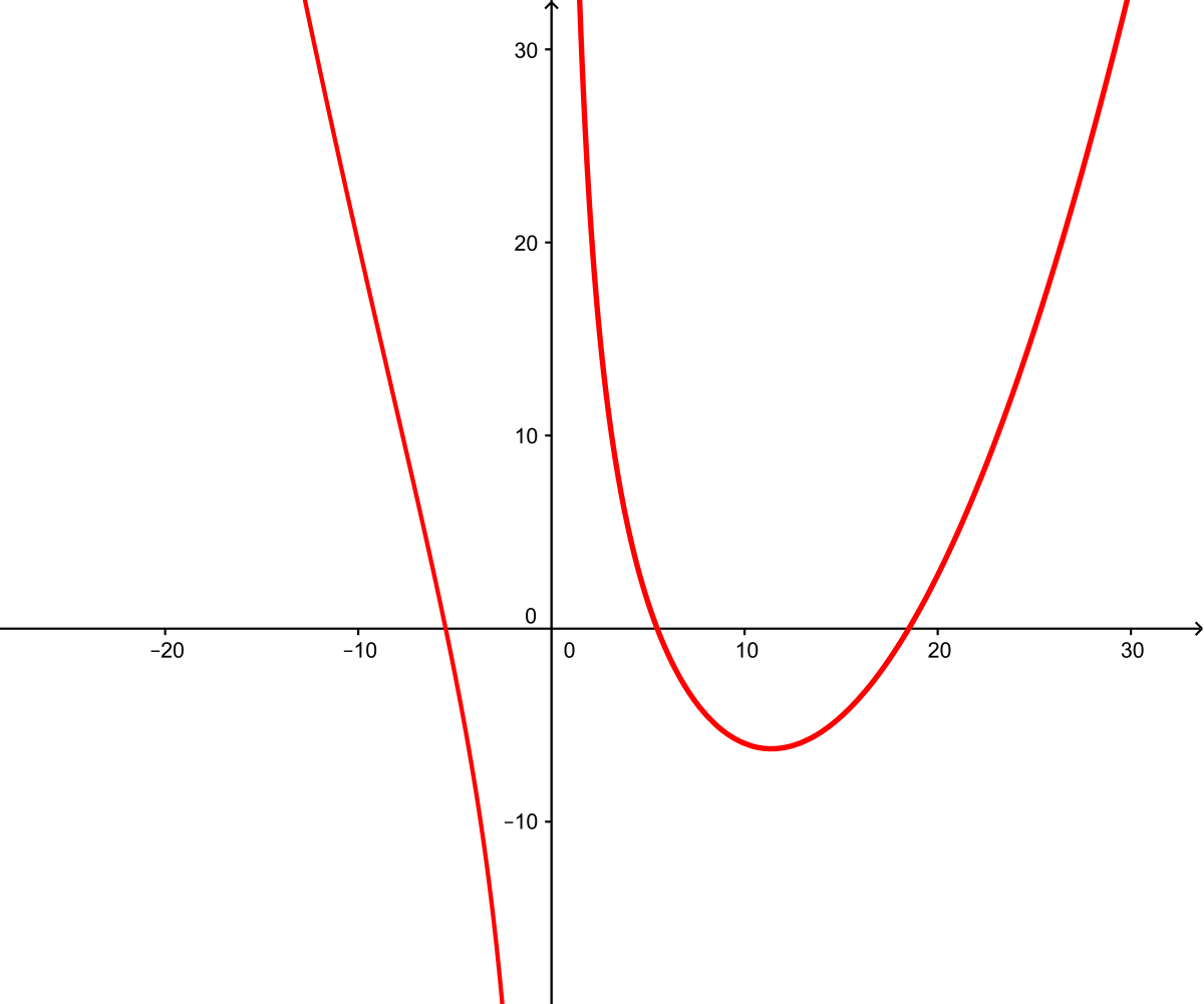
Figure 6. A Cartesian parabola
For constants \(n, a,\) and \(b,\) start with a parabola \(y=\frac{x^{2}}{n}\) with vertex D (D is the point \((0,0)\) to begin with). Place point E exactly \(a\) units above point D (E is the point \((0,a)\) to begin with). Then place the point A at \((b,0)\) and draw a line through A and E. This line intersects the parabola at two points, C1 and C2. For example, in Figure 7 below, \(n=10,\) \(a=3,\) and \(b=15\) (to begin with).
The parabola now ‘slides’ up and down in such a way that point E always remains \(a\) units above point D. Point A stays fixed so the line AE changes slope as E moves. Each possible location for the vertex creates new points C1 and C2 where line AE intersects the parabola. The locus of all the points C1 and C2 forms the two branches of the Cartesian parabola.
Figure 7. Constructing the Cartesian parabola. Instructions: Move the vertex D of the parabola up and down to see how the branches are formed. Move the sliders to adjust \(a, b,\) and \(n.\)
The equation for the two-branched Cartesian parabola, which will be derived later in this article, is the rational equation \[y=\frac{x^{2}}{n}-\frac{bx}{n}-a+\frac{ab}{x}.\] Notice that if you combine the fractions, you get a numerator of degree 3 and a denominator of degree 1, so this rational function has a vertical asymptote at \(x=0\) as well as a parabolic asymptote. Because of these features, the curve is a favorite with Precalculus instructors.
What makes this curve ‘simple’ is that it is based only on a line and a parabola, as opposed to, say, a graph of a cubic polynomial.
Gary Rubinstein (Stuyvesant High School), "Descartes’ Method for Constructing Roots of Polynomials with ‘Simple’ Curves - Simplest Curves for Higher Order Equations," Convergence (March 2016)


